
In one paragraph. The curled torus burps is a computational physics paper about a hypothetical sharp change in which flat space emerges from something more curled up. It uses a toy model of space as a network of dots and links, a close cousin of the published model called combinatorial quantum gravity. In that toy, a tube (a torus curled to four steps around) sits above the flat sheet in energy and is stable for now. The paper counts what it costs to start the change (12 units at the main setting, at every size tested), predicts how long the tube waits by counting its exits, watches the flat arrangement spread, seals the system to see where the released energy (the burp) goes, and counts what is left behind (about one four-dot scrap). A toy can show that a mechanism is possible or impossible within a class of models; that is the whole claim.
Everything you have ever seen happened in flat space: three directions you can move in. We know its rules well. What we do not know is how it came to be.
This paper is about a hypothetical change: space emerging sharply from something else. We want to understand that change, and how the two phases of being are related. We engage a toy model of dots and links and ask three questions: what does it take to start such a change, what comes out when it happens, and what is left behind.
Who is saying what
The project keeps four kinds of statement apart, and this edition tags them where it matters, so that a sentence is never quietly promoted from one kind to another. One more tag marks other people’s published work.
- EXACT Arithmetic, or a complete listing of every possibility. True of the model whatever a run does.
- MEASURED A simulation whose rules and predictions were written down before it ran, with its verdict. MEASURED, EXPLORATORY means a run that was not formally pre-registered: its prediction was only written into its configuration, or it is a closer look at runs already read.
- PUBLISHED Other researchers’ published results.
- OUR READING, UNVERIFIED A reading of a result, offered by the author and her AI assistants and checked by no physicist. THE AUTHOR'S CLAIM The author’s hypothesis about reality, stated as hers.
Numbers in square brackets point to the sources listed at the end.
CHAPTER 1 · THE PLACE WE START
We live in flat space, and we cannot rerun its birth
What was there before the Big Bang?
Nobody knows. This chapter sets up one way to study the question without a time machine: treat space as one arrangement of something deeper, and ask what kind of change could have produced it.
Side by side: the same ground in the technical edition, Sec. I, Introduction »
PUBLISHED Measured at the largest scales, our universe is flat: the angles of enormous triangles add up to what school geometry says they should, to within the precision of the best sky surveys [10]. It has three large directions. Its rules are known: general relativity for gravity and the shape of space, quantum mechanics for everything small.
What is not known is how such a thing comes to exist. Candidate theories say that space is not the stage on which everything happens but a phase of something deeper, the way ice is a phase of water. If that is right, there was a change, and changes come in two kinds.
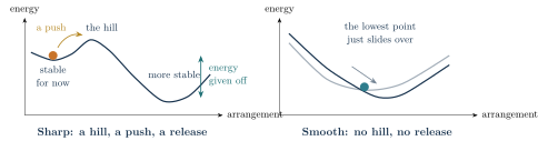
PUBLISHED Cool water, and nothing much happens until it reaches zero degrees. Then it freezes, giving off heat as it goes, with ice and water side by side for a while. Very clean water can even stay liquid below zero, stuck behind a hill it cannot climb on its own, until a jolt sets it off. Heat a fridge magnet instead and its pull fades away: no hill, no burst of heat, no moment when half of it has changed. Physicists call the first kind first order and the second continuous. Plainer words: sharp and smooth.
How do you tell which kind you have? PUBLISHED Let the system jiggle for a long time and count how often it turns up at each energy. A sharp change shows two humps with a valley between, because the system is almost always in one state or the other. A smooth change shows one hump.
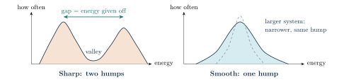
Two things make this hard. Small systems hide the hill: with only a few pieces, everything can flip at once, so even a sharp change looks like one broad hump. And the real test is whether the valley deepens as the system grows, which needs sizes nobody can simulate cheaply. Still, we set out a series of simulations that let us describe a sharp change of this kind in some detail.
Here is the author’s idea, in one paragraph. First, who is asking, and why. She is a software engineer, not a physicist, and also a startup founder and a foster mom, so her recreational time is scarce and the computing bills are her own. The project is called RecreationalPhysics anyway. Her reason is simple: she wants to map her intuition about how reality is organized onto what humanity knows about the universe.
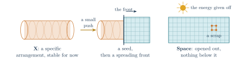
THE AUTHOR'S CLAIM Space is one settled arrangement of something deeper, which she calls X because nobody knows what it is. X was not chaos. It was a specific arrangement, stable for now, the way a reagent is stable until something gives it a push. The change that made space was sharp: it started at a seed, spread as a front, released a definite amount of energy that became matter and light, and left a remainder. Across the change the energy books balance.
That paragraph is a hypothesis, not a result, and nothing in a computer can prove it about reality. What a computer can do is take a model in which space is an arrangement of links, and ask whether a change of this kind can happen in it at all: whether there is a hill, how high it is, what comes down the far side, and what the far side is like. If the answer were no, the idea would have no home in that model. If the answer is yes, the idea gains a laboratory, and every number in it becomes a thing to check.
CHAPTER 2 · THE TOY
A published model of space made of links
Is space made of something smaller?
Some physicists think so. This chapter describes one published model, combinatorial quantum gravity, in which space is a network of dots and links and nothing else.
Side by side: the same ground in the technical edition, Sec. II, Model and exact results »
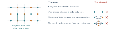
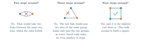
PUBLISHED The model is called combinatorial quantum gravity, built by Carlo Trugenberger, Christy Kelly and Fabio Biancalana [1, 2, 3]. It is a network of dots and links with no positions at all: a dot has no place, only neighbors. Figure 4 shows every rule it has. The mathematical word for such a thing is a graph; its dots are vertices, its links are edges.
The price list
PUBLISHED The model gives every arrangement an energy, and the energy is worked out by counting squares. Compared with an arrangement that has one square for every dot, every missing square has a cost. A single link may carry at most three squares; a link carrying a third one has one square too many, and every such surplus square has a cost of its own. Those two prices are the entire rule. To be clear, this energy has no meters or joules in it. We will just call its amount a unit, and leave the conversion of units into physical energy for a later paper. Everything below is in these units.
PUBLISHED A missing square costs 16 units. A surplus square costs 4λ units, where λ (lambda) is a number that sets the surplus price. It can be turned up or down, so we call it the knob. At exactly λ = 1 a surplus square costs 4, and the energy is then a measure of how curved the network is: a graph version of the curvature in Einstein’s equations of gravity. That is where the model’s name comes from, a theory of gravity built by combinatorics, the mathematics of counting. The published work also studies a simpler version with the surplus price switched off, λ = 0, where a link can carry a third square for free. Turning the knob to other values is our addition.
The whole point of the published program is to get general relativity, Einstein’s theory of gravity, back out of a network, so the curvature setting is the one that matters to it. At any other λ, however, the energy is still a perfectly good rule for a network, but it is no longer a curvature. So everything in this paper at λ ≠ 1 is a close cousin of combinatorial quantum gravity, not the thing itself.
We have not found published work that sets the surplus price to any value above 1 [11]. In print, as far as we have found, are the two settings just described and, in the text of two of the papers [2, 12], a version in which a third square is forbidden outright. So, barring a gap in our search, the approach taken here and what it turned up are new.

The one move
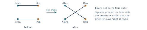
The network cannot leap to a new arrangement. PUBLISHED It changes by swapping partners: pick two links, Alice–Ben and Cara–Dan, and rewire them as Alice–Dan and Cara–Ben. Every dot keeps its four links and its group. Any swap that breaks the other rules is thrown out. That is the only move.
Warmth, and the bath
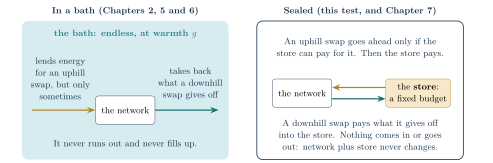
PUBLISHED A run of the model is a long chain of such swaps, each one proposed at random and then accepted or refused. A second number, g, decides which. It plays the part of temperature, and we call it the warmth. A swap that lowers the energy is always accepted. A swap that raises it by ΔE units is accepted only some of the time, with a chance of e−ΔE/g, where e is a fixed number, about 2.7: the bigger the cost, the rarer the swap, and the warmer the network, the more often it goes through. Picture the network sitting in a bath that lends it energy for an uphill swap and takes back whatever a downhill swap gives off. The bath is endless: it never runs out and never fills up. Lowering g is cooling the network. Time in a run is counted in sweeps: one sweep is two proposed swaps for every dot. Rules of this kind are the standard way to sample such a model; they are not a claim about how anything moved in real time.
The question the field asks, and reproduction as a starting point
PUBLISHED Start from a random tangle of links, cool it slowly, and watch. Does geometry condense out of the tangle sharply, with two humps, or smoothly? The published answers: with the full rule (λ = 1), smoothly [2, 3]; with the surplus price switched off (λ = 0), sharply, but the network breaks into many small closed pieces rather than one space [3, 4]. With a third square free, cooling packs in as many squares as the rules allow, and the most tightly packed arrangements close up on themselves; Chapter 3 shows what those pieces are. Kelly’s doctoral thesis [5] adds a hint for four links per dot: cooled and then warmed again, the network does not quite retrace its path, a small but persistent gap of the kind a sharp change leaves, though the thesis declines to call the evidence definitive.
MEASURED We repeated this before anything else.1 Our simulations land on the model’s published 2019 curve [2] to about half a percent at the same size, match exact averages at sizes small enough to list every possible arrangement, and reproduce the sharp change into closed pieces with the surplus price off. Then we measured how much energy the change gives off as the tangle orders, at several sizes, with the rules written down first.
| Setting | Dots | Energy given off per dot as the tangle orders |
|---|---|---|
| Surplus price off (λ = 0) | 48 | 10.3 |
| 64 | 11.3 | |
| 96 | 12.5 | |
| Full rule (λ = 1) | 36 | at most 1.65 |
| 64 | at most 1.51 | |
| 100 | at most 1.30, and falling |
MEASURED With the surplus price off, the energy given off is large and grows with size, but the cold state is a pile of closed pieces, not a space. With the full rule, which does make a space, there is one hump at every size we ran, and any energy given off is small and shrinking. Settings of 1.25 and 1.5 gave the same picture. We got the same answer the published work did, and added the comparison across sizes that the 2019 paper said was out of reach.
CHAPTER 3 · THE PHASE BEFORE
What if what came before space was not random?
What existed before space?
The author's hypothesis is that it was not nothing and not chaos, but a specific curled-up arrangement. This chapter builds a stand-in for that arrangement inside the toy model.
Side by side: the same ground in the technical edition, Sec. II, Model and exact results »
The published question starts from a random tangle. This program asks a different one: what if what came before space was not random at all, but a specific arrangement, stable for now, with energy to give? That question is the focus of everything that follows. To ask it in the toy, we first need to say what space looks like in a network with no positions, and what the alternative to it could be.
Directions
Space, at its simplest, is a set of large directions: directions you can keep walking in. Figure 7 shows how to find them in a network that has no positions.
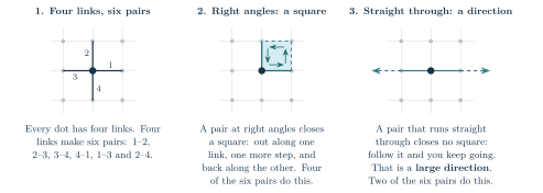
A grid with no edges
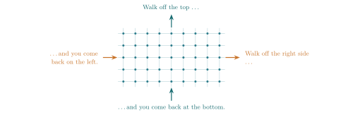
A grid drawn on paper has edges, where the dots run out of links. The toy removes the edges.
Curling
If a direction is not large, what else can it be? Small: curled up on itself.
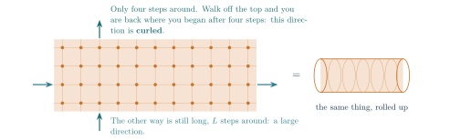
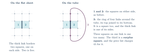
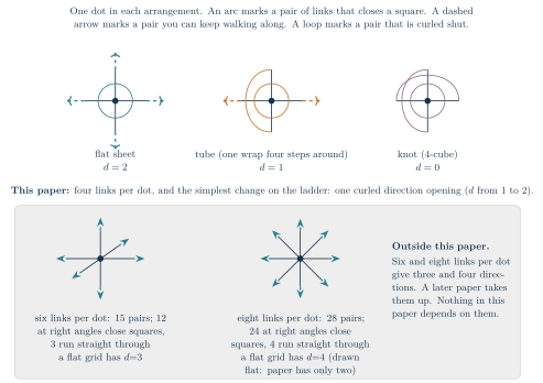
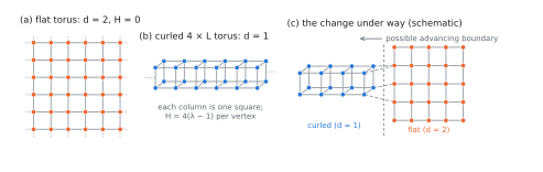
Curl both ways around to four steps and every dot reads d = 0: a closed sixteen-dot knot called the 4-cube. Most of the closed pieces of Chapter 2 are these knots. Figure 12 puts the three arrangements side by side.
The ladder
EXACT Put the three arrangements side by side: flat sheet, tube, knot. Each curls one more direction than the one before, so we call them the rungs of a ladder. The price list of Chapter 2 gives each rung its bill, per dot:
| flat sheet | tube | knot | |
|---|---|---|---|
| Directions curled | none | one | both |
| Squares per dot | 1 | 1¼ | 1½ |
| saved on squares, at 16 each | 0 | 4 | 8 |
| Surplus squares per dot | 0 | 1 | 2 |
| paid for surplus, at 4λ each | 0 | 4λ | 8λ |
| Bill per dot: paid minus saved | 0 | 4(λ − 1) | 8(λ − 1) |
| at λ = 1.25, where a surplus square costs 5 | 0 | 1 | 2 |
Curling is a trade between the squares it gains and the surplus it pays for, and the knob decides which side wins.
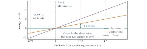
This is the first thing the toy teaches. EXACT At the curvature setting, curled and flat cost the same, so a curled arrangement has nothing to give and no reason to open. For a change of this kind to happen anywhere in this family of rules, the knob has to sit above 1. There, a tube that opens into a flat sheet gives off exactly 4(λ − 1) units per dot.
That release is what the rest of this paper is about, so it gets a name of its own. The author calls it the burp: the energy given off, and by extension the event that gives it off, a quiet wait, a start, a spreading change and a definite release.
PUBLISHED The standard account of a stable-for-now state giving way calls its central calculation “the bounce” [8]. The two names point at opposite ends of the event. The bounce is about the start: it gives how often a seed of the new state appears, in a quantum system that tunnels through its hill. The burp is about the end: what comes out. And the toy has no tunneling. Its tube goes over the rim, with energy lent by the bath or handed to it as a push, never through it.
OUR READING, UNVERIFIED The author reads the extra price as a curling cost: the rule is still curvature, plus a charge on every tightly curled link, and that charge is exactly what a burp gives back. Where space is smooth nothing is curled tight, so the charge vanishes and only curvature remains. That reading is hers, and it is unreviewed.
Stable for now: is there a window?
Energy to give is not enough. Supercooled water has energy to give and sits there. For the tube to be a stand-in for X it must be stuck: every single swap away from it must cost energy. EXACT At 18 dots the model is small enough to list every allowed arrangement: there are 26, counting arrangements that differ only in the names of their dots as one. Among them, arrangements above the flat sheet from which every single swap costs energy exist for knob settings between 1 and 1.6, and for no larger setting. So the knob has a window, and a narrow one.
The stand-in
Our stand-in for X is therefore the tube. At λ = 1.25 it sits exactly one unit per dot above the flat sheet. It is a stand-in and not X: it has one large direction where space has three, its curled direction is always four dots around, and it lives in a network of a few hundred dots. What it shares with X is the shape of the idea under test: a specific, curled, stable-for-now arrangement with energy to give.
The running example
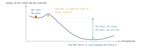
Take a tube of 96 dots: four around, 24 along. At λ = 1.25 it holds 96 units above the flat sheet. That is the burp on offer. We will follow this tube through the rest of the paper so that the amounts stay concrete. It is a running example, not an invented history: the evidence comes from hundreds of repeated runs and, where possible, from counting every allowed move.
Now the question that decides whether any of this is a story at all. Ninety-six units are waiting to come out. What does it cost to start?
CHAPTER 4 · THE OBSTACLE
What does it cost to start?
What could have set off the Big Bang?
Unknown. In the toy model a change of this kind needs a push, and the push can be counted exactly: twelve units, the same at every size tested.
Side by side: the same ground in the technical edition, Sec. III, The cost of leaving »
Before any number, consider what the number could mean. If the push needed were tiny, a few units, then any warmth at all would set the tube off, and it would not be stable for now. If the push were as large as the burp itself, 96 units for our tube and more for a bigger one, then starting the change would cost what the change gives back, and the cost would grow with the size of the tube. Nothing small could ever start something large. A sharp change of the kind pictured in Chapter 1 needs a middle answer: a push that is small, and that does not grow with the size of the thing being pushed, so that a bigger tube releases a bigger burp from the same spark. A fixed push and a growing release is the condition for a runaway.
So: is the cheapest exit from a perfect tube small, fixed, or neither?
Pricing the cheapest exit
EXACT Start from a perfect tube and try every swap the rules allow, the one move of Chapter 2. Each one breaks some squares and removes some surplus, and the price list gives its cost. Most are expensive. Some cost nothing: they twist the tube around itself without changing any dot’s neighborhood, so they do not count as leaving. Among the swaps that do leave, two kinds are cheapest. Call them route A and route B. Here are their bills at λ = 1.25, where a surplus square costs 5:
| Route A | Route B | |
|---|---|---|
| Squares broken | 2 | 4 |
| charged, at 16 each | + 32 | + 64 |
| Surplus squares removed | 4 | 10 |
| refunded, at 5 each | −20 | −50 |
| The bill | 12 | 14 |
Route A is the cheaper at this setting; the two tie at λ = 4/3, and B is the cheaper beyond. (For readers who want every exit listed with its formula, the technical paper [9] has them in Section II.)
The cheapest way out of the tube costs 12 units.
Twelve. Not 96, and not 2. For our 96-dot tube the push is an eighth of what comes out; for a 288-dot tube, which holds 288 units, the same 12 is a twenty-fourth. EXACT The cost of the cheapest single swap does not depend on how long the tube is, because a swap only touches a handful of neighboring dots; the burp does, because every dot contributes one unit. That is the middle answer the change needed, and it is arithmetic.
Is 12 really the floor?
One cheap exit from the perfect tube is not the same as no cheaper exit anywhere nearby. The free twists lead to other arrangements with the same energy, and one of those might have a cheaper door. EXACT So the calculation followed every free twist, at six sizes from 48 to 288 dots, until no new arrangement appeared. At each size there are exactly three reachable arrangements, counting arrangements that differ only in the names of their dots as one; every one has the same menu of exits, and the cheapest costs 12. This is a complete finite computation, conditional on the enumeration code being right, not a proof for every conceivable size: at a control size of 32 dots the pattern is different, which is a reminder not to extrapolate.
The test from the other side
Arithmetic says nothing below 12 can leave. Does 12 suffice? To find out, take the bath away and hand the tube an exact budget and nothing more (Figure 16), a standard way to simulate at a fixed total energy [7].
MEASURED, EXPLORATORY Try budgets of 4, 8, 10, 11, 11.5, 12, 13 and 16 units, eight runs at each budget at each of five sizes from 48 to 192 dots: 320 runs in all, each 12,000 sweeps long.
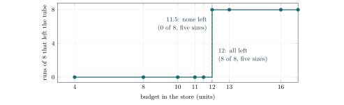
EXACT The lower half of this staircase is a theorem of the model at these sizes: with no exit cheaper than 12 and a store that cannot go negative, a budget below 12 can only pay for free twists. The upper half is an observation about this protocol and duration.2 MEASURED, EXPLORATORY Together they say that the wall is local, exactly 12 units high at λ = 1.25, and the same at every size tried, while what waits behind it grows with the system.
Why we went here. This is the pivot of the whole paper. Suppose the push had grown with the size of the tube, so that a tube twice as long needed a push twice as large. Then no single spot could start the change: something would have to push the whole tube at once, and the picture of a seed and a spreading front would fail in this model. We would have had to look for this kind of change in another one. A fixed, cheap push against a growing release is the condition under which something small can start something large.
CHAPTER 5 · THE WAIT
How long before the door opens, and what kind of waiting is it?
What is a metastable state, or false vacuum?
A state that is stable for now: it lasts until chance hands it enough energy to leave. This chapter predicts how long the toy's version waits, and checks the prediction.
Side by side: the same ground in the technical edition, Sec. IV, The first exit »
A rim of 12 says what a push must be. It does not say when a tube left to itself will go. For that we put it back in the bath of Chapter 2 and let the network jiggle at warmth g. A swap that climbs the rim, costing 12, is accepted with chance e−12/g: warmer, and the rim is cleared more often.
A lottery with counted tickets
Now the wait becomes a lottery, and every ticket can be counted. EXACT In one sweep the computer proposes two swaps for every dot, 2N in all for a tube of N dots, each one picked at random from every swap there is. How many of those proposals are exits?
Take route A. A tube of N dots has 3N different route-A swaps: three for every dot, so a longer tube has more ways out. But a longer tube also has more swaps of every other kind, and those grow faster, as N times N. So the chance that any one proposal lands on a route-A exit is 3 in 2N, smaller for a longer tube. A sweep makes 2N proposals. Multiply the two and the length cancels: \[2N \;\times\; \frac{3}{2N} \;=\; 3 .\] A sweep offers three route-A exits on average, whatever the size of the tube. A longer tube has more exits, each one is harder to hit, and with two proposals per dot in a sweep the two effects balance exactly. The same count for route B gives two.
Each offer of A is accepted with chance e−12/g, each offer of B with chance e−14/g. So the chance of leaving in any one sweep is 3 e−12/g + 2 e−14/g, and the mean wait is one divided by that, with nothing fitted: \[\text{mean wait} \;=\; \frac{1}{3\,e^{-12/g} + 2\,e^{-14/g}} \quad\text{sweeps.}\] At g = 1.5, the warmth used for most runs below, that is 845 sweeps. Chemists know this shape as an Arrhenius law. Here both of its ingredients, the height of the rim and the number of tries per sweep, are counted from the arrangement rather than fitted to the data (the technical paper [9], Section II, gives the formula for any λ).

Does the tube keep the appointment?
MEASURED, EXPLORATORY The first test ran twelve conditions at λ = 1.25: six warmths from g = 1.4 to 2.5, two sizes, sixteen tubes each, with measured waits from about 30 sweeps to about 2,500. The prediction written down for this test counted route A only, which makes the predicted wait a little longer than the full formula does: 994 sweeps at g = 1.5, where the full formula gives 845.
Averaged over the twelve conditions, the measured wait came within 2 percent of the predicted one. One condition at a time the match is looser: they range from 29 percent shorter than predicted to 62 percent longer (Figure 19). That is the scatter a lottery gives: with only sixteen tubes, their average wait lands, by chance alone, about 25 percent above or below the true average. The two sizes also differ. The 144-dot tubes sit near the full formula, and the 64-dot tubes waited longer. This exploratory test cannot say whether that is chance, which is one reason for the stricter test below.
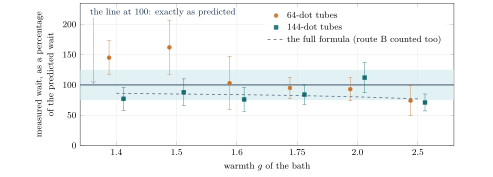
MEASURED A stricter, pre-registered test then counted every single accepted swap in 240 further runs across six settings of λ and size, and compared the first exits with the full formula, both routes. All 240 first exits were observed, and their mean arrived when the formula said it would in every cell, within the scatter expected from that many runs.
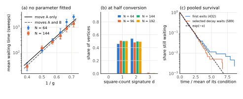
What kind of waiting
If the chance of escape is the same on every attempt, the waits are memoryless. It is like rolling a die until a six comes up: twenty rolls without one do not make a six any likelier on the next roll, and a tube that has waited a long time is no nearer to leaving. One sign of a memoryless wait is that the waits spread out by about as much as their average. MEASURED That check was pre-registered, and it passed at every size in the main run. MEASURED, EXPLORATORY Checked afterwards, the whole distribution of first exits is consistent with that picture too, panel (c) above. The time to a detected change looked different, with a tail the first exits do not have. Chapter 9 finds out why.
MEASURED One more thing the move-by-move count revealed: the first swap out does not always lead anywhere. Think of that first swap as a door opening. About a third of the time the door closes again, and the tube goes back to being a perfect tube. Only 56 to 68 percent of first exits went on to a real change, with no trend in λ. The formula predicts when the door opens, not the departure.
A caution about the clock
OUR READING, UNVERIFIED The clock here counts attempted swaps, not seconds. One sweep offers any one neighborhood a way out about 1/N as often as a clock that gave every neighborhood its own fixed rate would. On that fairer clock the wait would fall as 1/N, and a longer tube would go sooner. The model has no time in it; which clock is “right” is not a question it can answer, and a later paper adopts the fairer one.
Why we went here. If the measured wait had disagreed with the counted lottery, something larger than a single swap would be holding the tube shut, and 12 would have been the wrong number. It agrees. The rim is the single swap, and the lottery is the whole explanation of the first exit.
CHAPTER 6 · THE CHANGE
What takes shape on the other side
Can space change phase, the way water freezes?
In the toy model it can: a patch of the new arrangement appears and grows while the old one is still there beside it. This chapter watches that happen and says what the pictures do and do not prove.
Side by side: the same ground in the technical edition, Sec. V, The conversion »
Chapter 5 was about the start: the first swap out, and whether it holds. This chapter is about what comes next: how the change spreads through the tube. It spreads fast.
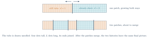
The natural picture is a zipper. One spot of the tube opens, and the opening runs along the tube the way a zipper runs along a jacket. The slider, the tab you pull, is the boundary: behind it the tube has already opened into flat sheet, and ahead of it the tube is still closed. Physicists call a moving boundary like this a front. To find out whether the zipper picture is right, we need an instrument.
EXACT The fastest instrument is the direction count d of Chapter 3. Dots still in the tube read d = 1; dots on a flat sheet read d = 2; a melted, disordered dot reads 0 or 3 and up. The program marks every dot and also keeps a progress meter that runs from 0 (all tube) to 1 (all flat). It takes a snapshot of the whole network at three stages fixed in advance: when the meter first reads a quarter, a half and three-quarters. These are stages of the change, not times on the clock, and there is nothing special about them. They were fixed beforehand so that nobody could pick a moment because its picture looks persuasive. The predictions were scored at the half mark, where tube and sheet are most evenly matched and anything in between would have the most room to show.
MEASURED At λ = 1.25 and g = 1.5, thirty tubes at each of four sizes, run twice with fresh random numbers, and three predictions written down first: a memoryless wait; at least 80 percent of dots in one of the two signatures at the half mark; and at least 70 percent of the flat-like dots in one connected region, on average. All three held at every size in both runs. At the half mark 98.8 to 99.8 percent of dots read as tube or sheet. The other two snapshots were recorded but not scored. Read afterwards, they say the same: 98.8 to 99.7 percent at a quarter, and 98.5 to 99.5 percent at three-quarters. Something organized was happening, early, midway and late, with almost nothing in between.
What the count cannot vouch for
A jacket found open along one long stretch could have been unzipped from one spot, or from two spots whose openings ran into each other before anyone looked. So one large open region is weaker evidence than one zipper. MEASURED The averages passed the 70-percent rule at every size, but individual runs did not always. Of the thirty runs at 64, 96, 144 and 192 dots, 0, 2, 4 and 9 fell below it in the first set, and 0, 1, 3 and 5 in the second. A separate pre-registered test of a simple one-front law came out NOT ESTABLISHED: 21 of 59 tubes that started converted in several patches, mostly at the warmer bath. The honest description is that one connected flat-like region usually dominates by the half mark, and that the change often starts in more than one place: more than one zipper.
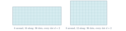
Nor does a count certify a geometry. EXACT A single swap from a perfect tube can produce dots that read d = 2 while their links carry one, two, two and three squares, which no dot on a flat sheet does. Two buildings can contain the same number of rooms and have different floor plans. And a grid six steps around and enormously long reads flat at every dot while keeping one direction short. The paper therefore calls d = 1 and d = 2 curled-like and flat-like signatures. When it says the curled direction opened, it means only that the four-step curl is gone, not that both directions were shown to grow large. The second has not been measured.
A stronger look at the finished wiring
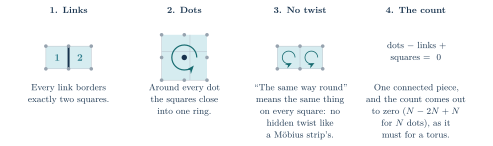
EXACT For the 120 saved final networks at λ = 1.05, the smallest knob setting in the map of Chapter 9, the check was done the hard way, from the wiring itself (Figure 23). All 120 passed. Those endpoints are tori, established from the wiring and not from a count. Their two ways around were not measured.
The energy comes out exactly
MEASURED When a tube finishes as a perfect flat sheet, the energy given off is exactly one unit per dot at λ = 1.25: the arithmetic of Chapter 3, now measured. In 24 to 28 of 30 runs per size the release was within one percent of that. The rest settled on sheets with small defects, 8 to 45 units’ worth read from their wiring, and held back that much. The ideal gap is exact; how much of it comes out depends on where the network stops.
Why we went here. A sharp change means two arrangements side by side with a front between them, not everything softening at once. Only a snapshot in the middle of the change can test that, and only an instrument fixed in advance keeps us from choosing the snapshot we like.
CHAPTER 7 · CLOSE THE LID
Where does the energy go when it has nowhere to go?
Where did the energy of the Big Bang come from?
In the author's hypothesis the change itself released it, the way freezing water gives off heat. In the toy model that release, the burp, can be counted exactly and followed when nothing is allowed to leave.
Side by side: the same ground in the technical edition, Sec. VI, Sealed system: the reservoir and the relic »
Apart from the budget test of Chapter 4, every run so far sat in the bath, and the bath carried the released energy away as fast as it appeared. If a change like this made all of space, there was no outside for its energy to go to. So seal the system again, as in Chapter 4, and watch what the burp does to its own surroundings.
EXACT The sealed system of Chapter 4 had one store. Here there are C stores beside the network, each holding a non-negative number of units. Every proposed swap picks one store at random: an uphill swap is refused unless that store can pay; a downhill swap deposits its release there. Nothing enters or leaves, so network plus stores is constant to the unit, and it was checked to be constant in every run.
Return to our 96-dot tube, holding 96 units. Put 12 more in a store and seal the lid. The account reads 108. Suppose the change runs and leaves one 14-unit scrap in the sheet, as Chapter 8 will show it often does. The network has gone from 96 to 14; the stores have gone from 12 to 94.

The surroundings can spoil the ending
Here is the twist. The released energy is now in the stores, and the stores pay for uphill swaps. Energy that has nowhere to go can buy swaps that break the very squares the change has just made. How much damage depends on how many stores there are. PUBLISHED Many stores share the release thinly, like a large cold room; few stores concentrate it, like a small hot one.
MEASURED Pre-registered: tubes of 64, 96 and 192 dots, seven choices of C from a single store to two per dot, twenty runs at each setting, 420 runs. The outcomes were classified by rules fixed beforehand: sheet-like if at least 90 percent of dots read d = 2 with almost no melted dots; melted if 15 percent or more read as disorder; stalled if both orders sat side by side with nothing melting; in between otherwise.
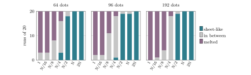
MEASURED A bonfire with a threshold, as the pre-registered verdict put it. Where the heat has room, the change feeds itself to completion; where it does not, the heat melts what the change made. Melted means the dots lose their neat two directions and go back to being linked any old way, which is the random phase the published model starts from. The switch-over moves in step with size, as a release of one unit per dot shared among the stores predicts. OUR READING, UNVERIFIED A rough energy budget puts it near one store per three dots; the measured crossover sits between one per four and one per two, which is as fine as the grid can say. That estimate assumes the stores settle into a thermal balance, and individual store balances were not saved, so it is a budget, not a calibrated thermometer.
MEASURED No run stalled with tube and sheet side by side and nothing melting. Our reasoning said that outcome needs a temperature at which the two arrangements are equally happy, and no such temperature exists in this model. A single stalled run would have refuted that reasoning. Said carefully: none appeared in 420 runs of 30,000 sweeps on this grid of C. That is not a proof that the two can never coexist.
Why we went here. What the burp turns into, and whether the energy books balance across the change, only have meaning in a sealed system. In a bath the burp leaves and nothing can be asked of it. The sealed box is where the balance becomes a measurement.
CHAPTER 8 · WHAT REMAINS
A scrap of the old arrangement
Is anything left over from before the Big Bang?
In the toy model something is: about one small scrap of the old arrangement survives each change. Whether anything like it exists in reality is not something a toy can say.
Side by side: the same ground in the technical edition, Sec. VI, Sealed system: the reservoir and the relic »
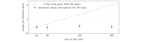
Almost every sheet that formed in a cold sealed box kept something: four dots of the old curled arrangement that the change swept past without opening. A remainder raises one question first: does it grow with the space? A remainder that grows in step with the space is a fixed share of everything, big enough to be some of what a universe is made of. A remainder of fixed size is a speck. The prediction, written down before the measurement, was that it grows.

MEASURED Eighty fresh runs in the coldest box, two stores per dot, pre-registered: tubes of 64, 96, 192 and 288 dots. The count of scraps per finished sheet was 0.90, 0.85, 1.05 and 0.95, with a spread of about 0.2 to 0.4 either way across the twenty runs at each size. A straight line drawn through them is flat, within that scatter. About one scrap per box, however long the tube.
Where does it sit, and why one?
It is tempting to call the scrap the place where two fronts met and left a seam. MEASURED That was pre-registered and tested: the scrap sits neither opposite the start nor at it, and a randomization check that moves it to every position along the tube finds nothing special about where it landed. We do not know why the count is about one in this protocol. The technical paper [9] says so under “not claimed.”
What the scrap does afterwards
This paper stops at the count. Three questions follow from it, and they are the subject of the author’s next paper: does a scrap last, or heal away, when the sheet around it is kept warm or is cooled; does a change that starts in several places at once leave more of them; and if so, is the leftover a speck or a share. The short version: how many scraps survive depends on how the change started and how fast the sheet cooled, and more than one prediction written down beforehand failed.
Why we went here. The change leaves a remainder in almost every run, at every size. The pre-registered test asked the one question that decides what kind of thing it is, and the answer, fixed size, is not the one the author predicted. It is reported as prominently as the results that went her way.
CHAPTER 9 · THE MAP
Turning the knob
How do you test an idea about the universe with a simulation?
By turning one knob at a time with the rules written down first, and publishing every setting, including the ones that failed. This chapter is that map.
Side by side: the same ground in the technical edition, Sec. VII, Dependence on λ »
Everything so far was at one setting of the knob, λ = 1.25, chosen in advance. A single setting proves little: a result that only holds at one carefully chosen number is the kind of thing the project’s rules forbid. So the whole stretch of the knob was run, from 1.05 to 1.45 in steps of 0.05, at four sizes, thirty tubes per cell, with the rules fixed first. Then it was run twice more with 120 tubes per cell and fresh random numbers. Each run carries a detector that decides when the change has happened. It watches the tube for its first 200 sweeps to learn what an unchanged tube looks like, and only then starts checking, so it cannot record a change earlier than that. The end of this chapter returns to what this costs.
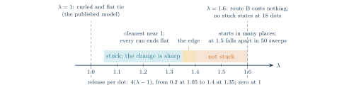
MEASURED Three things the map shows. First, the tube is stuck at every setting from 1.05 to 1.35 and at none from 1.40 up, and wherever it is stuck the change keeps the character of Chapter 6: 95 to 100 percent of dots in one signature or the other at the half mark, one connected region holding most of the flat-like dots. Second, the mean wait follows the counted lottery of Chapter 5 over a hundred-fold range of waiting times with nothing fitted, drifting above it only where the 200-sweep watch cannot record shorter waits, and running 15 to 43 percent long near λ = 1, where the direct move-by-move count finds no excess. Third, the change is cleanest near the published setting and gets messier as the knob turns: at 1.05 every one of 120 tubes ended as a perfect flat torus, at 1.25 about 88 percent did, at 1.35 fewer than half, and beyond the edge the change starts in several places at once in most runs and ends mostly on a sheet with defects.
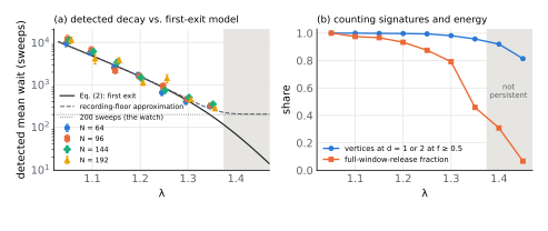
OUR READING, UNVERIFIED There is a trade here. A larger λ means a larger burp per dot but a less patient X and a messier birth; a smaller λ means a cleaner change that releases less. The release is exactly 4(λ − 1) per dot and vanishes at the published setting, so this family of models has no setting with a large release and a quiet, clean X at once. PUBLISHED At the published setting itself, the model’s author has proposed that patches of the network can sit stuck in a different arrangement [6]; the questions asked here could be put to those patches too.
Three verdicts, all inconclusive by the letter
MEASURED Each of the three maps was scored against rules fixed before it ran, and each failed one of them: the first on a band for the spread of waits that, with thirty tubes, turned out to be not much wider than ordinary run-to-run scatter, so a cell could fall outside it by chance alone; the second on an energy check that compared a window average with an exact final energy and was tripped by the sheet’s own thermal jitter; the third on the spread of waits again, in four cells, two of them on a single tube recorded as waiting 24 and 76 times the predicted mean (neither of those two was a wait, as the end of this chapter shows). Three runs, three different criteria tripped, and the physics reading the same each time. The verdict stays inconclusive, because that is what the rules said, and the measurements stand as the result.
The long waits that were not waits
MEASURED One loose end from these maps looked alarming for a while. The third map recorded two tubes waiting 24 and 76 times the predicted mean, which a memoryless wait all but forbids. A dedicated pre-registered test of 10,000 tubes then counted too many long waits and returned the verdict TWO POPULATIONS. It also found a fast share, 12 to 23 percent of tubes that seemed to change at once, and 190 tubes the detector never caught.
Was something hidden in the model, or was this the detector? It was the detector (Figure 30). For its first 200 sweeps the detector only watches, to learn how much a resting tube jiggles, and then it sets its bar at three times that jiggle. A tube that changes during the watch teaches it that large swings are normal.
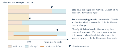
MEASURED, EXPLORATORY Every run saved two readings that do not depend on the detector’s bar: how far the tube had converted when the watch ended, and when a quarter of it had converted. Read afterwards from those saved rows (a reading made after the fact, not a pre-registered test), the puzzle comes apart. The 190 tubes never caught had all finished at least three-quarters of the change inside the watch. The two extreme waits were tubes already 75 and 88 percent converted when the watch ended, resting on a sheet with defects. The fast share is tubes whose first exit came inside the watch, about as many as the counted lottery says there should be. And the test’s yardstick for a typical wait, taken with the fast share included, came out too short, which pushed ordinary long waits past its cutoff.
The verdict stands as scored; what it reported on was its own detector. Three long waits in one group of 4,000, at λ = 1.30 and 64 dots, were not explained this way, so we replayed that whole group move for move from its saved starting numbers, this time recording everything, with the rules for reading it written down first. MEASURED One of the three was the detector again. The other two looked like perfect tubes every time the replay looked, which was once every five sweeps. So we replayed them once more and looked after every single sweep. MEASURED, EXPLORATORY One had sat, perfect, for about twelve times the average wait. The other had slipped out for three sweeps between two looks and come back, about seven average waits in, so its long wait was the spacing of the looks. At no sweep did any tube hold more squares than a perfect tube, which a second curl would need. MEASURED Neither written guess about the three held (a hidden second curl; the detector three times over). Timed with no detector at all, the 4,000 first exits follow the counted lottery to within 7 percent, and one comes later than ten average waits, which chance allows about one time in six.
Why we went here. The project’s first success condition is no cherry-picking: a family of rules may be explored, but only along knobs fixed in advance, and every setting run is published. The map is that rule applied, and it also locates where the stand-in for X stops being stable for now.
CHAPTER 10 · THE EDGES
Where the simulations stop, and what lies past each edge
Can a computer simulate the beginning of the universe?
Not the real one. This chapter lists exactly how far these simulations go, where each stops, and what lies past each edge.
Side by side: the same ground in the technical edition, Sec. VIII, Discussion »
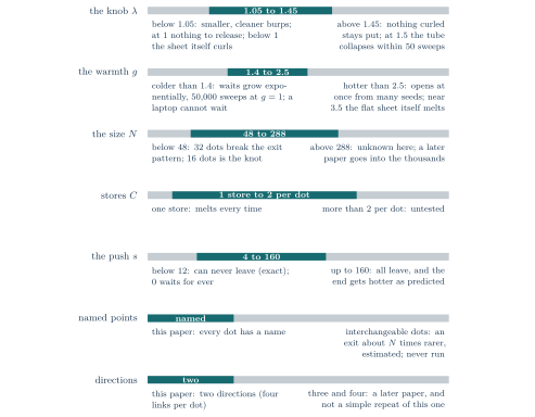
Every knob the toy has was turned only so far. This chapter is the honest map of the box: for each knob, what was run, why it stopped there, and what is on the other side, with the kind of knowledge marked. “Unknown” means no one has looked.
The knob λ: 1.05 to 1.45
Below 1.05 the burp gets smaller and cleaner, not longer-awaited. EXACT The wait saturates as the knob approaches 1 (the counted lottery gives about 8,300 sweeps at 1.05 and about 14,000 at 1.001), while the release shrinks to nothing at exactly 1, where curled and flat tie and the tube is no longer above anything. Below 1 the ladder flips. MEASURED, EXPLORATORY In a rehearsal the author calls the backwards reaction, a perfect flat sheet at λ < 1 sat at zero for hundreds to thousands of sweeps and then curled, one direction first, releasing energy in steps that landed on the exact rungs of the ladder. Above 1.45, MEASURED at 1.5 the tube falls apart within 50 sweeps in every run; EXACT at 1.6 route B costs nothing and at 18 dots no stuck state above flat exists; by a knob setting of 5 to 10 the model behaves as one with a third square simply forbidden. Nothing curled is stable for now out there.
The warmth g: 1.4 to 2.5, with the maps at 1.5
EXACT Colder, the wait grows like e12/g: about 50,000 sweeps at g = 1 and nearly three million at g = 0.75. MEASURED, EXPLORATORY At g = 1, two of four tubes were still tubes after 30,000 sweeps. A laptop cannot wait long enough below about 1, which is why the knob stopped there. Hotter, the tube opens almost at once and from many places, and near g ≈ 3.5 the flat sheet itself melts into the random phase; that melting point is the one the reservoir estimate of Chapter 7 used. How that melting point moves with the size of the sheet is taken up in a later paper; until then every warm result carries a size caveat.
The size N: 48 to 288 dots
The upper limit was run time on one laptop and the choice to spend compute on repeats rather than size. EXACT The exit count was certified at 48 through 288; the control at 32 dots breaks the pattern, and 16 dots is the knot. MEASURED The front’s speed fell roughly as the size to the power −0.7, so longer tubes take longer to finish. OUR READING, UNVERIFIED Whether the wait itself grows, stays flat or falls with size depends on the clock the model does not fix (Chapter 5). The technical paper claims nothing beyond 288. Networks into the thousands of dots are the subject of a later paper on the scrap.
Stores C: one to two per dot
MEASURED A single store melts every tube; two per dot leaves clean sheets with one scrap. Colder boxes than two per dot were not tried. The store balances were not saved, so they cannot be turned into a calibrated temperature after the fact.
The push s: 4 to 16, then 12 to 160
EXACT Below 12 nothing can leave by single swaps, at the certified sizes; a tube with nothing to spare waits for ever, which is now a permanent test in the code. MEASURED, EXPLORATORY Above, pushes of 12 to 160 units at 64 dots all left, and the hotter the box the more disordered the sheet it ended with, with the ending predicted from the model’s equilibrium curve before the run: 0.97 squares per dot measured against 0.95 predicted at the smallest push, 0.81 against 0.81 at the largest. Give it far more and it melts.
Named or interchangeable dots
OUR READING, UNVERIFIED Every run treats dot 17 as a different thing from dot 41. If instead two networks that differ only by renaming count as one, as identical particles do, every energy stays the same and so does the 12, but each exit from the perfect tube would be accepted about N times less often, because the tube has many symmetries and the state one swap away has two. The waiting time would then grow with size instead of staying flat. The knob exists, was decided on, and was not turned for this paper.
Directions: two
Four links per dot give two directions. Six and eight links give three and four (Figure 12), closer to the three directions of space, and they are the subject of a later paper. The tease: a curled direction in three dimensions does not open the way the tube does, and the reason is partly exact and partly still open.
The route
The published route starts from a random tangle; this paper starts from an ordered tube. MEASURED Both were run. From randomness at λ ≥ 1: one hump, no sign of a release at these sizes. From the tube at λ > 1: a hill, a push, a burp. The two routes are different questions, and the toy gives them different answers.
CHAPTER 11 · WHAT WE HAVE LEARNED, AND WHAT COMES NEXT
A mechanism we can price, and two questions it opens
Is this a theory of where the universe came from?
It is a hypothesis, with one mechanism tested in a toy model and no physicist's review yet. This chapter says what was learned and what would have to come next.
Side by side: the same ground in the technical edition, Sec. VIII, Discussion »
Return one last time to the 96-dot tube. Its excess energy is exact: 96 units. The cheapest way out is exact: 12 units, the same at every size certified. The counted lottery predicts when it first leaves, and the tube keeps that appointment over a ninety-fold range of waits. Halfway through, 99 dots in 100 belong to one arrangement or the other. When it finishes flat, it gives off exactly one unit per dot, and sealed, the energy is followed to the unit into stores and into a four-dot scrap. The whole chain holds at every setting of the knob from 1.05 to 1.35.
What the toy shows about this kind of change
OUR READING, UNVERIFIED What the toy shows is that a graph energy one coefficient away from a published model of emergent geometry contains a change with the shape of the idea in Chapter 1: a specific curled arrangement, stable for now, that opens sharply from a seed with a fixed push, releases a definite and growing burp, and leaves a fixed remainder. It shows that this change does not exist at the curvature setting and needs the knob above 1. It shows that the release has to have somewhere to go or it undoes the change. And it shows that the remainder, from one seed, is a speck.
What it does not show is anything about reality. A toy can show that a mechanism is possible or impossible within a class of models; that is the whole claim. THE AUTHOR'S CLAIM The author claims that reality works this way, and people can argue. The model’s part is to make the claim concrete enough to be wrong in specific ways, and several of those ways have now been tried: the remainder did not grow, the single-front law was not established, three maps were inconclusive by their own rules, and a test that reported a second population of waits turned out to be reporting on its own detector.
What another researcher can build on
Some parts are exact or complete finite listings: the ladder, the 12, the three reachable arrangements, the topology of 120 endpoints. Their scope is the stated rules, sizes and the correctness of the code, which is tested against independent calculations. Other parts are measurements with variation between repeated runs, where a hundred dots in one run are not a hundred experiments. Tests written down before the data are marked pre-registered; the Arrhenius scan, the push threshold and the endpoint-energy reading are exploratory and say so. Interpretations are the author’s and her assistants’ and have not been checked by a physicist.
Even what to count is a choice. The simulations count named dots. Counting each wiring once, with the names removed, leaves every energy alone and changes the rates, most for the symmetric arrangements that are easiest to calculate with and that nothing is ever in. That knob is decided and not yet turned.
What the next round of this experiment should record
Time every tube from its first sweep, with no watch, and save every exit and return. Measure both ways around the finished torus as the size grows. Record each store’s balance, so that the bath’s temperature can be read and not estimated. Hold out the largest size and predict it from the smaller ones before it runs.
What comes next
The question that began the work survives its first test. Can an organized arrangement give way sharply, release energy and leave a remainder? In this small laboratory it can, and the first step can be priced to the unit. Two things were left standing at the edge of what this paper measured, and each has a paper of its own coming, with its predictions written down first.
The scrap. A scrap is the only thing in the new space that still carries the old arrangement, so the next paper, What the burp leaves behind, asks what it takes to keep one. MEASURED One result: the scrap counted here is not permanent. Cool the new sheet slowly enough and it heals away, while another kind of leftover survives every cooling we could run.
Three directions. The tube has one open direction, and space has three, so the paper after that, How curled directions open, runs the same rules with six links per dot. MEASURED One result: the tube’s trick does not carry over. Here one fixed push set off the whole change. There each curled direction sits behind its own wall, and one push has never opened them all.
A push of twelve units opens a tube. What opens a space?
Continuing into the technical paper
This edition follows the technical paper [9], which holds the equations, tables, uncertainty calculations and full references. Every number above is taken from it or from the project’s record, and the kinds-of-statement tags follow the project’s own rule that no statement is promoted from one kind to another without a dated note saying why. Its sections run in the same order as the chapters here: the model and its exact results (Chapters 2 and 3), the cost of leaving (4), the first exit (5), the conversion (6), the sealed system (7 and 8) and the dependence on λ (9).
A few translations for the next step
| In the paper | What to keep in mind |
|---|---|
| N | Number of dots. The running example uses N = 96. |
| 4 × L | Four steps around the short wrap and L around the other, L even and above 4. 4 × 4 is the knot. |
| λ and g | Lambda sets the price of a surplus square and so the whole ladder; g is the bath’s warmth, which sets how often an uphill swap is accepted. |
| H = 16(N − S) + 4λX | The price list: S squares, X surplus squares. Zero on the flat sheet; 4(λ − 1) per dot on the tube. |
| ΔE‡ = 32 − 16λ | The rim: the cost of route A, 12 at λ = 1.25. Route B costs 64 − 40λ. |
| d | The direction count: pairs of links at a dot that close no square. Sheet 2, tube 1, knot 0. A counting signature, not a certified geometry. |
| f | The progress meter, 0 for the tube and 1 for the sheet. Disorder raises it too. |
| Arrhenius law | Uphill events becoming much rarer as the bath cools, as e−cost/g. Here its two ingredients are counted, not fitted. |
| Memoryless | The chance of leaving is the same on every attempt, like rolling a die until a six comes up; a long wait so far makes leaving no nearer. |
| Metastable | Stable for now: every single move out costs energy. The map’s edge near 1.37 is where the wait drops below the watch, not where that stops being true. |
| Microcanonical | Sealed: energy conserved, the temperature read off the stores rather than imposed. |
| Pre-registered | The prediction and the rules of the test were committed before the run. Exploratory runs say so. |
| 95% interval | A range from a statistical procedure that, under its assumptions, covers the truth 95 times in 100. |
Where the evidence is recorded
The technical manuscript and its methods supplement are in the recorded repository version, and the supplement maps every claim to code, configurations and result files. Experiment labels in that record: T7 and T8 (the decay and the map), T9 (the sealed reservoir), T10 and T11 (the scrap and its position), T22 (exits counted move by move), T38 (the long-wait test). The questions teased above, what the scrap does afterwards, larger networks and more directions, have their own labels in the record and their own papers. The push threshold covers 48 to 192 dots and the exit enumeration 48 to 288; neither extends to other sizes.
Disclosure
The author used Claude (Anthropic) and ChatGPT/Codex (OpenAI) to assist with code, analysis and writing, and is responsible for the result. This edition was drafted with Claude from the corrected manuscript and the project’s record. Its analogies and pictures introduce no new experiments or evidence. No physicist has reviewed any of it.
Sources
- C. A. Trugenberger, Combinatorial quantum gravity: geometry from random bits, J. High Energy Phys. 09 (2017) 045, arXiv:1610.05934. Cited as in the technical paper.
- C. Kelly, C. A. Trugenberger, and F. Biancalana, Self-assembly of geometric space from random graphs, Class. Quantum Grav. 36, 125012 (2019), arXiv:1901.09870.
- C. A. Trugenberger, Networks as the fundamental constituents of the universe, J. Phys. Complex. 6, 042001 (2025), arXiv:2512.17676.
- A. Gorsky and O. Valba, Interacting thermofield doubles and critical behavior in random regular graphs, Phys. Rev. D 103, 106013 (2021), arXiv:2101.04072.
- C. Kelly, Emergent geometry and discrete curvature in random graphs, Ph.D. thesis, Heriot-Watt University (2022), https://www.ros.hw.ac.uk/handle/10399/4591.
- C. A. Trugenberger, Dark matter and dark energy in combinatorial quantum gravity, arXiv:2409.09385 (2024).
- M. Creutz, Microcanonical Monte Carlo simulation, Phys. Rev. Lett. 50, 1411 (1983). Cited as in the technical paper; we have not read it in full.
- S. Coleman, Fate of the false vacuum: semiclassical theory, Phys. Rev. D 15, 2929 (1977). Described here from general knowledge of the paper; we have not read it in full.
- E. Smith, The curled torus burps: activated escape and conversion in a graph model of emergent geometry, technical manuscript, 10 October 2026, in the project repository.
- Planck Collaboration, Planck 2018 results. VI. Cosmological parameters, Astron. Astrophys. 641, A6 (2020), arXiv:1807.06209.
- The written search behind this sentence, 10 October 2026: where we looked, with what terms, and what came closest. File
docs/reading/notes/2026-10-10_prior_work_lambda_above_one.mdin the project repository. - C. Kelly and C. A. Trugenberger, Combinatorial quantum gravity: emergence of geometric space from random graphs, arXiv:1811.12905 (2018).
Sources 1 to 8 carry the same numbers as in the technical paper [9]; 9 to 12 are this edition’s own.
Notes
- One published 2025 figure from the same group [3] disagrees with ours over one stretch, but it also disagrees with that group’s own 2019 curve [2], so it is a question for them and is recorded as open. ↩
- Why not run a hundred tubes at each budget instead of eight? Our reasoning, from the exact counts, is that it would add little. Below 12, leaving is impossible, which is arithmetic, and no number of runs can strengthen it. At 12 or more, the count of Chapter 5 says a perfect tube is offered, on average, three exits costing 12 in every sweep, and with 12 in the store the first one offered is paid for at once. A run that stayed put for 12,000 sweeps would itself be the surprise. The runs check that count; they are not estimating an unknown chance. ↩
The big questions, and what this work can honestly say
What was there before the Big Bang?
Nobody knows, and this work does not settle it. It tests one hypothesis, the author's: that space is one settled arrangement of something deeper, and that before the change there was a different, specific arrangement, curled up and stable for now. A toy model shows that such a change can happen in a network of dots and links, with a countable push and a countable release. That is a possibility shown in a toy, not evidence about the real universe.
Where did the Big Bang come from?
One hypothesis, tested here only in a toy model: the hot early universe is the energy released when an earlier arrangement gave way and space opened out, the way water gives off heat when it freezes. In the toy the release can be counted exactly and grows with the size of the system, while the push that starts it stays small and fixed at every size tested.
What was there before time?
This paper cannot say. The toy model has no time in it: its clock counts attempted moves, not seconds. In the author's wider hypothesis, which this paper does not test, what came before space had order but not time as we experience it.
Is space made of something?
Possibly. In the published model this work builds on, space is a network of dots and links with no positions at all, and flat space is one arrangement of that network. Whether real space is like that is an open research question.
Is this an accepted theory?
No. It is a hobbyist's hypothesis, tested on a toy model with the predictions written down first, written with AI assistance and not yet reviewed by a physicist. The paper says exactly what was and was not shown.
Quick answers
What is “The curled torus burps” about?
It is a plain-language edition of a computational physics paper by Emily Smith. It asks what a sharp change from one specific arrangement into flat space would look like, and tests each part of that picture in a toy model made of dots and links: what it costs to start, how long the wait is, what takes shape, where the released energy goes, and what remains.
What is combinatorial quantum gravity, and is this it?
Combinatorial quantum gravity is a published model, built by Carlo Trugenberger, Christy Kelly and Fabio Biancalana, in which space is a network with no positions at all and the energy is a count of squares that acts as a curvature. This paper uses a close cousin of that model, not the model itself: it turns one knob, the price of a surplus square (λ), above the published value of 1.
What is a curled torus?
A torus is a grid that wraps around in both directions. Curl one direction until it is only four steps around and you have a tube. In the model the tube has one large direction where the flat sheet has two, and it sits 4(λ − 1) units of energy per dot above the flat sheet: one unit per dot at λ = 1.25.
What is the burp?
The burp is the energy given off when the tube opens into the flat sheet. For a clean change it is exactly 4(λ − 1) per dot, so it grows with the size of the tube, while the push needed to start it does not.
How much energy does it take to start the change?
Twelve units at λ = 1.25: the cost of the cheapest partner swap out of a perfect tube, counted exactly, the same at every size from 48 to 288 dots. In 320 sealed runs, no tube left with a budget below 12 and every tube left with 12 or more.
How long does the tube wait before it starts?
Count the exits a sweep offers, multiply by the chance each is taken, and you predict the mean wait with nothing fitted. Across twelve conditions the measured mean wait divided by the predicted one averaged 0.98. The waiting is memoryless, like rolling a die until a six comes up.
What is left behind after the change?
About one four-dot scrap of the old arrangement per sheet, holding 14 units, whatever the size of the tube, in the sealed runs with the most room. What the scrap does afterwards is the subject of the next paper.
Does this show how the universe began?
No. A toy can show that a mechanism is possible or impossible within a class of models; that is the whole claim. The clock in the simulation is a sampling rule, not physical time, and no physicist has reviewed the work.
Was AI used to write this?
Yes. The author used Claude (Anthropic) and ChatGPT/Codex (OpenAI) to assist with code, analysis and writing, and is responsible for the result. The predictions for the main tests were written down before the runs.
What this page is about
what came before the Big Bang, emergent spacetime, combinatorial quantum gravity, graph model of space, curled torus, metastable state, false vacuum decay, activation energy, first exit time, memoryless waiting time, nucleation and front, sealed system (microcanonical), Creutz reservoir, relic defect, pre-registration, Markov chain Monte Carlo, decompactification.
Sign the guestbook
Leave a note, a question or a correction. The guestbook runs on e-mail, as in 1996: the button opens your mail program with your entry filled in, and you press send.
Your address is used only to reply to you and, if you tick the box, to tell you about the next paper. Or skip the form and write to emilysmithcreate@gmail.com.
How to cite this page
Emily Smith, The curled torus burps: A small push, a large release, and the question of what survives (plain-language edition), 10 October 2026. https://sidenerdapps.com/mainnerd/01thecurledtorusburpsPL/
@misc{smith2026curledtorus,
  author = {Smith, Emily},
  title  = {The curled torus burps: A small push, a large release, and the question of what survives},
  year   = {2026},
  month  = oct,
  note   = {plain-language edition},
  url    = {https://sidenerdapps.com/mainnerd/01thecurledtorusburpsPL/}
}