The curled torus burps

I. Introduction

Side by side: in the plain-language edition this is Chapter 1, The place we start »

Combinatorial quantum gravity (CQG) [1, 2, 3] treats space as a network: a discrete Ricci curvature, summed over a graph, favors configurations with geometric structure. Published equilibrium studies ask how geometry emerges from a random phase, and they do not all simulate the same set of graphs: Ref. [2], Sec. 4, describes a restricted bipartite simulation in which no edge has surplus squares, whereas Ref. [3] discusses the uncapped curvature action, and Ref. [4] finds first-order behavior in a related model with no surplus price and no fixed bipartition. They are context, not checks of the same model. Kelly’s thesis [5], p. 219 and Fig. 4.58, reports small four-regular hysteresis loops over N = 50–500 but declines a definitive first-order inference.

We ask instead how a specified ordered arrangement escapes and converts at fixed coupling. It is a tube: a torus curled to a period of four edges in one direction. It is stable for now in the energetic sense: at the sizes enumerated (Sec. II) no single move out of the perfect torus lowers its energy for the λ studied, yet lower states exist. We call its energy-releasing conversion a “burp.” Removal of the four-cycle signature does not establish macroscopic decompactification: the reconstructed original endpoints retain a six-edge shortest noncontractible loop as N grows. This is a deformation next to CQG, not a CQG allotrope in the sense of Ref. [6].

Why deform CQG at all? At λ = 1 an edge carrying three squares costs exactly what an edge carrying two costs, so the flat torus, the curled torus and the 4-cube are degenerate: conversion between these ideal states releases no energy (equal energies need not imply equal free energies). The coefficient λ lifts that degeneracy and changes nothing else: the states, the moves and the hard-core rule are those of CQG. For λ > 1 the ground states are the arrangements with two squares on every edge, a condition that fixes neither connectedness nor topology, and each curled direction costs a known energy per vertex. The family is therefore a controlled laboratory for a change between two ordered arrangements in which the barrier, the release and the relic can each be counted exactly, and λ → 1 connects it to CQG.

Every kinetic statement below (waiting times, barriers, fronts) is about one Markov chain: the local edge switch used to sample the model [2], with Metropolis acceptance and an ordered-pair proposal that are our choices (Ref. [3] uses Glauber acceptance). Detailed balance makes the Boltzmann distribution stationary but does not show mixing at our sizes, and we do not claim that the chain is the physical time evolution of emergent space. Endpoint energy differences depend on the Hamiltonian, not the proposal rates. The cheapest single escape cost also depends on the allowed move set; it is not a measured barrier to completing the change. Rates depend on the proposal and acceptance rules, including how waiting time scales with size (Sec. II).

A plain-language edition with diagrams accompanies the source (Methods); its chapters are cited as “PL, Ch. n” where a concept is developed at greater length.

II. Model and exact results

Side by side: in the plain-language edition this is Chapter 2, The toy and Chapter 3, The phase before »

Diagrams for this section are in PL, Chs. 2 and 3.

A state is a simple undirected four-regular graph on a fixed labelled bipartition, N/2 vertices on each side, obeying the hard-core rule: no two vertices share more than two neighbours [2, 3]. Connectedness is not enforced. The energy is a price list on squares (four-cycles). With S the number of squares, S_e the number on edge e, and \(X=\sum_e(S_e-2)_+\) the surplus squares on edges carrying more than two, \[\begin{aligned} H &= 16\,(N - S) + 4\lambda X\\ &= 4 \sum_e \bigl[(2 - S_e) + \lambda\,(S_e - 2)_+\bigr], \end{aligned} \tag{1}\] so a missing square costs 16 and a surplus square 4λ. The hard-core rule limits S_e ≤ 3: two squares on edge uv through the same neighbour w of v would give u and w three common neighbours. At fixed dimensionless coupling g > 0, which acts as a temperature in the units of H, the target is π(G) ∝ e^−H(G)/g, and a valid symmetric proposal is accepted with probability min(1,e^−ΔH/g). At λ = 1 this is the CQG curvature action, which Ref. [3] (its Eq. (21)) writes as a sum of the curvature κ over every vertex and each of its neighbours, \[H=-4\sum_v\sum_{w\sim v}\kappa(v,w),\] so that each edge appears twice. On these bipartite graphs κ(v,w) = −(2 − S_vw)₊/2, which gives \(H=4\sum_e(2-S_e)_+\) with each undirected edge counted once. For λ ≠ 1, H is not this curvature action.

Zero is the floor (exact). Since 2 − S_e = (2 − S_e)₊ − (S_e − 2)₊, Eq. (1) can be rewritten as \[H=4\sum_e\bigl[(2-S_e)_+ +(\lambda-1)(S_e-2)_+\bigr]\] which shows H ≥ 0 for λ ≥ 1: no state lies below flat. For λ > 1, H = 0 if and only if every edge carries exactly two squares; at λ = 1, at least two. Flat lattice tori are ground states, and so are disconnected unions of them, so topology must be checked separately.

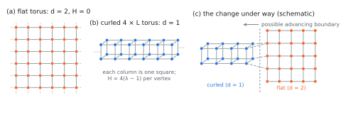
The ladder (exact). Periodic bipartite tori need even periods. Curl one direction of a torus to period four and the walk around it becomes a square, which puts a third square on every edge of each wrap-around 4-cycle. For even L > 4 the 4 × L torus therefore has S = 5N/4 and X = N, and sits H/N = 4(λ − 1) ≡ ε above a zero-energy state. Curling the other direction too gives the 4-cube (4 × 4), with H/N = 8(λ − 1): each curled direction costs 4(λ − 1) per vertex in these ideal products (Fig. 1). A decay that ends with residual graph energy H_f releases Q = εN − H_f, which is εN only for a zero-energy endpoint.

Counting signatures. A vertex has six pairs of incident edges. Let d(v) be the number of pairs that close no square: 2 on a flat lattice torus, 1 on a one-curled torus, 0 on the 4-cube. This is not a geometric dimension. Under the hard-core rule a pair closes at most one square, so with q_v squares through v, d(v) = 6 − q_v and \(\sum_vd(v)=6N-4S\). The recorded conversion coordinate is \[f=\frac{5N/4-S}{N/4}=\overline d-1,\] which equals the fraction of vertices at d = 2 only when no signature other than d = 1 and d = 2 is present. Melting raises f too, and even d = 2 does not certify flat order (a valid single switch at N = 64 produces vertices whose incident edges carry [1,2,2,3] squares, not [2,2,2,2]). We therefore call d = 1 curled-like and d = 2 flat-like counting signatures.

Other stuck states at N = 18 (exact enumeration). Enumerating all 26 graph classes and solving the inequalities H > 0 and ΔH > 0, linear in λ, for every valid single switch, with no grid in λ, gives precisely two strict local minima above the ground state on λ ≥ 1: (S,X) = (21,12) on the open interval 1 < λ < 8/5 and (22,16) on 1 < λ < 4/3. This small-system certificate is not a large-N phase diagram.

The way out: counting the exits. The chain’s one move swaps one partner each between two vertices of the same side (an edge switch preserving the bipartition), accepted by the Metropolis rule with the hard-core rule enforced. A proposal draws two edges one after the other, each uniformly from the 2N edges (a vertex of one side and one of its four slots). There are 4N² equally likely ordered proposals, and every switch is proposed in two ways. A sweep is 2N attempts.

From the perfect 4 × L torus, at the sizes enumerated below, the cheapest switches are of two kinds. Move A (ΔS = −2, ΔX = −4) costs 32 − 16λ and can be made in 3N ways, hence 6N ordered proposals; move B (ΔS = −4, ΔX = −10) costs 64 − 40λ and can be made in 2N ways, 4N proposals. A sweep therefore offers move A 2N × 6N/4N² = 3 times and move B twice, whatever N. Weighting each offer by its acceptance gives a two-channel approximation to the mean first-exit time with nothing fitted, \[\tau_{AB}(\lambda, g) = \bigl[3 e^{-(32 - 16\lambda)/g} + 2 e^{-(64-40\lambda)/g}\bigr]^{-1}, \tag{2}\] with A the cheaper for λ < 4/3 and both costs positive in the kinetic range used here. For a constant full per-attempt hazard p the exact first-exit law is geometric, with mean 1/(2Np) sweeps; the exponential is its small-p approximation.

First, N/2 switches change neither S nor X: each reconnects two neighbouring columns at opposite points, twisting the torus globally without leaving its energy. Breadth-first enumeration exhausts the neutral classes reached this way at λ = 1.25 for N = 48,64,96,144,192,288. At each size there are three side-preserving isomorphism classes, all with the same full list of moves and minimum exit cost 12. Every valid switch is checked at each representative and every neutral target belongs to the exhausted list; since relabellings map switches bijectively, this certifies closure at these sizes, not for arbitrary L. Second, Eq. (2) leaves out every dearer exit. Each costs at least 10 more than the cheaper of A and B for 1.05 ≤ λ ≤ 1.45, but those that break two distant edges at once are offered a number of times per sweep that grows in proportion to N (87 at N = 192). Counted exactly, they add at most 2% to the exit rate at the g = 1.5 conditions of the decay maps, and 16% at the hottest point of Fig. 2(a) (g = 2.5, N = 144), within its error bar. Third, that Eq. (2) does not depend on N is a property of the proposal, not of the barrier: the chain draws its two edges from the whole graph, so any one region is offered a way out about 1/N as often per sweep. On a size-fair clock, which gives every region the same chances at every N (N/96 sweeps to the unit, as in the companion paper on the relic), the waiting time falls as 1/N.

III. The cost of leaving

Side by side: in the plain-language edition this is Chapter 4, The obstacle »

At λ = 1.25 the cheapest move out of the perfect curled torus, move A, costs ΔE^‡ = 12. This opens the door: it is a first-exit cost, not a proven minimum of the maximum energy along a complete conversion path (the minimax barrier of energy-landscape analysis [10]), and whether an excursion then grows or falls back is a separate question (Sec. IV). The neutral-class enumeration of Sec. II makes 12 a lower bound at the enumerated sizes; an energy-conserving test asks whether it is also enough (PL, Ch. 4).

To seal the system, that is, to make it isolated with its total energy strictly conserved (microcanonical dynamics), we replace the external bath at fixed g by a Creutz reservoir [7]: C stores of nonnegative energy. Each valid candidate move selects one store uniformly; the move is refused if that store cannot pay ΔH, and otherwise the store’s energy changes by −ΔH, so that \(E_{\rm tot}=H+\sum_iE_i\) is conserved. Stores and edge proposals are both selected globally: a seed is a total activation budget, not energy deposited at a chosen vertex. The recorded maximum drift of \(E_{\rm tot}\) is zero in all T9 runs at λ = 1.25 (an observed check, not a claim about bitwise arithmetic at arbitrary λ).

A push that does not grow with size (exploratory). With one store initially holding s ∈ {4,8,10,11,11.5,12,13,16}, the torus left its initial (S,X) values in 8 of 8 runs at each tested s ≥ 12 and in 0 of 8 at each s ≤ 11.5, for each N = 48,64,96,144,192 (320 runs of 12,000 sweeps). The lower half of this staircase is exact at these sizes: by the neutral-class certificate of Sec. II all moves that change the energy cost at least 12, so nonnegative stores with total budget below 12 cannot leave the basin. The upper half is an observation, dependent on protocol and duration. Eight successes give a two-sided exact 95% binomial interval of [0.631,1] at an individual setting (zero of eight gives [0,0.369]), and the runner checks (S,X) once per sweep, so its success flag measures escape, not completed conversion. The push is fixed while the available ideal-state energy decrease εN grows with the system.

IV. The first exit

Side by side: in the plain-language edition this is Chapter 5, The wait »

Table I defines the clocks used below, which are not interchangeable; PL, Ch. 5, develops the rate count.

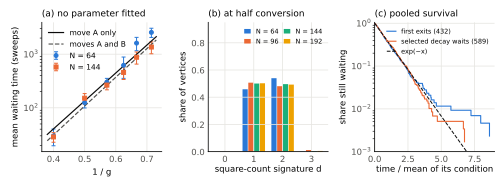
Testing the count (exploratory). The prediction was written into the run’s configuration before it ran, but not pre-registered. Over twelve conditions (g = 1.4 to 2.5, N = 64 and 144, 16 runs each) and a ninety-fold range of times, the ratio of the measured mean waiting time to the move-A term of Eq. (2) has a plain mean of 0.98, every ratio between 0.71 and 1.62 [Fig. 2(a)]. The scan reuses each replica’s seed across couplings, so its cells are not independent; the direct count below is the rate test.

The direct count (T22). Forty further runs in each of six cells (λ = 1.05,1.10,1.25; N = 64,96) count exits attempt by attempt. All 240 first exits are observed, and their means are consistent with Eq. (2) in the exponential-model 95% intervals in the Supplemental Material. An opened door is not a departure, though: many exits fall back into the curled torus. Of the 240 runs, 239 reach f ≥ 0.25 before the cap, and for these completed runs the reciprocal of mean exits per run is 0.56–0.68, with replica-bootstrap intervals spanning roughly 0.45–0.78 across cells. This estimates successful departures per counted exit under the f ≥ 0.25 commitment rule. It is not a correction factor for the exit rate, which would need independent excursions and the time spent in failed ones and in growth.

A memoryless wait? (exploratory). A constant chance of exit per sweep gives a memoryless, exponential wait. The coefficient of variation is a coarse diagnostic, not sufficient to establish memorylessness. Dividing each time by its condition’s mean and pooling over conditions, the 432 first exits we recorded give a Kolmogorov–Smirnov distance D = 0.035 from the unit exponential (nominal p = 0.53; shared-stream caveat in Methods) [Fig. 2(c)]. The 240 of them counted move by move (T22, above) are consistent with an exponential using the mean of Eq. (2), nothing estimated (p = 0.85). This does not establish exponential tails in each cell. Detected-decay waits show stronger departures, including the later T38 tail-test failures (Sec. VII).

V. The conversion

Side by side: in the plain-language edition this is Chapter 6, The change »

The decay itself was pre-registered: at λ = 1.25, g = 1.5, thirty decays at each of N = 64,96,144,192, with the adjacency read when the conversion fraction first crossed 25, 50 and 75%. The predictions, averaged across replicas, were a memoryless waiting time (coefficient of variation between 0.7 and 1.3) and, at half conversion, at least 80% of vertices at d ∈ {1,2} and the converted vertices in one piece holding at least 70% of them. All three component tests hold at every size and on two independent sets of seeds (Table II). They show a dominant connected flat-like region in the evolving graph at half conversion, not unique nucleation or a single moving interface. The measured means show no clear decrease with N over these sizes; detected waits need not have the same size dependence as first exits.

The same pre-registration listed λ = 1.5; there the torus does not persist under the tested protocol at g = 1.5 (its number of squares per vertex falls to 0.95, below the flat torus’s 1, within 50 sweeps in every replica), and no verdict was applied. A separate pre-registered test of whether a coarse law of a single front governs these decays (T12; 64 decays at g = 1.5 and 2.0, under Metropolis and Glauber acceptance) came out NOT ESTABLISHED: 21 of the 59 that nucleated converted in more than one patch, mostly at the warmer coupling, and the front’s rate per sweep fell roughly as N^−0.7 (on the size-fair clock, N^{+ 0.3}).

The 25 and 75% snapshots, recorded but not registered, give the same picture: the mean share at d ∈ {1,2} is 0.988–0.997 and 0.985–0.995 across the eight cells, against 0.988–0.998 at 50% (PL, Ch. 6).

What is released. The energy difference between the ideal states is exact; what a given decay releases depends on where it ends. After settling, 24 to 28 of 30 decays per size have a window-averaged release within 1% of ε per vertex. This energy criterion alone does not certify torus topology. The other endpoints hold defects, read from their wiring: most often combinations of small defects of 8 to 45 units, and less often the four-point relic of Sec. VI, a closed loop of four vertices at d = 1 with S = N + 1 and, in its commonest form, X = 6, costing 24λ − 16 (14 at λ = 1.25). Whether these states are stable or only slow is not known. The energy criteria were written after endpoints had been inspected, so this part is exploratory. Under them the full two-state classification holds at N = 64,96,192, while one N = 144 run fails because its state changes inside the final measuring window. The prespecified waiting and morphology criteria pass at all four sizes in both sets of thirty runs; a passing component test is not a passing combined classification.

A count is not a geometry. At λ = 1.05 all 120 saved endpoints of the map of Sec. VII have zero energy. Filling every square as a face and checking two faces per edge, a cyclic vertex link, connectedness, orientability and Euler characteristic zero certifies torus topology for all 120 graphs. A retrospective translation-lattice reconstruction now also checks every adjacency. Each is a square-grid quotient isomorphic to a 4 × L tube with a two-site seam shift. Its shortest noncontractible loop is six edges; a shortest independent loop has length L = N/4 = 16,24,36,48. The six-edge loop does not make it a rectangular 6 × L torus.

The same retrospective audit covers all 3,521 zero-energy saved endpoints in the reached subset of T60 (35 cells, including N = 288). Of these, 3,446 are connected tori with shortest loop six, 73 are disconnected closed square surfaces, and two are connected nonorientable surfaces with Euler characteristic zero, hence Klein bottles. Surface checks include cyclic vertex links; width alone cannot certify topology. The two rows outside the reached subset also end at zero energy after settling, but are excluded from this denominator. The supplement gives the selection, algorithm and per-file certificates. This is a finite-sample result, not an arbitrary-size theorem.

A seam shift of 2m sites gives a zero-energy torus with shortest loop 4 + 2m (verified for m ≤ 4, L ≥ 24), so the energy neither favors nor opposes widening beyond six: it prices four-cycles and nothing longer. Counted as lattice wrappings (not isomorphism classes, and not a statement about what the dynamics reaches), zero-energy tori with shortest loop six are 8.5% of the 236 wrappings at N = 192 and 5.2% of 387 at N = 288. Every switch out of a zero-energy torus costs energy: by exhaustive listing at N = 48 and 96, at least 16λ from the torus with shortest loop six (no square broken, four surplus squares made) and at least 32 from those with shortest loop eight to twelve. The observed endpoints are the nearest one.

A separate equilibrium scan at λ = 1.25 has a single energy-distribution peak over the tested sizes and couplings and is INCONCLUSIVE under its stated rules. Neither that finite-size observation nor the kinetic conversion studied here establishes a thermodynamic first-order transition.

VI. Sealed system: the reservoir and the relic

Side by side: in the plain-language edition this is Chapter 7, Close the lid »

Sealed, the released energy has to go somewhere, and the C stores of Sec. III are the only place (PL, Ch. 7).

Reading a temperature off the stores. At λ = 1.25, ΔH = −16ΔS + 5ΔX is an integer. The initial T9 stores contain 0 or 12, and allowed exit costs include 12 and 25, with greatest common divisor one, so store energies have no common increment coarser than one, though this does not prove every allocation can be reached. If in equilibrium with a graph at fixed coupling (canonical), an unbounded store with levels kδ has a geometric energy distribution, whose mean u_D is tied to the coupling by \[u_D(g)=\frac{\delta}{e^{\delta/g}-1},\qquad g=\frac{\delta}{\ln(1+\delta/u_D)}.\] For δ = 1, u_D(3.5) = 3.024, and u_D = 0.5 corresponds to g = 0.910. We report the coupling inferred this way only as a proxy valid at equilibrium: store histograms were not saved, so their distribution cannot be checked.

Each move and its reverse are equally likely, so the uniform distribution over reachable graph-and-store states at fixed total energy is stationary, though not shown to be reached. If all integer bath allocations at energy \(M=E_{\rm tot}-H(G)\ge0\) are accessible, their number is \(\Omega_C(M)=\binom{M+C-1}{C-1}\), and each graph’s weight is multiplied by this count. Changing C therefore changes the entropy as well as the thermal response.

Enough room, or not. The seed sits in one of C stores, and C sets the reservoir’s heat capacity (C = 1,N/16,N/8,N/4,N/2,N,2N; N = 64,96,192; twenty runs each of 30,000 sweeps; 420 runs). With too little room the run ends in the registered class “melted” (at least 15% of vertices at d = 0 or d ≥ 3) in 17 to 20 of 20 runs for C ≤ N/16 and in 9 to 16 of 20 at C = N/8. At C = N/4 most runs end in neither class. That class is damage and not the random phase. A sealed run holds εN + s, and with X ≥ 0 the squares per vertex cannot fall below 1 − (εN + s)/16N, about 15/16 here; the 154 runs so classified end with 0.94 to 1.00 squares per vertex, against about 0.13 in the random phase. With enough room, C ≥ N/2, the “sheet” counting criterion holds in 18 to 20 of 20; 18/20 and 20/20 successes have exact 95% binomial intervals [0.683,0.988] and [0.832,1]. The criterion requires f ≥ 0.9, at least 90% at d = 2, and less than 5% at d = 0 or d ≥ 3; it is not a topology test. The observed crossover lies between N/4 and N/2 on this coarse grid. A conditional equilibrium energy-balance estimate at crossover coupling g_m would be \[C^*\simeq\frac{\varepsilon N+s-U_{\rm graph}(g_m)}{u_D(g_m)}.\] Taking g_m ≃ 3.5 and neglecting seed and residual graph energy gives N/3.024: an approximate energy budget, not a calibrated crossover prediction. Stores have no upper capacity, so a small bath heats; it does not fill up. No sustained stall with both signatures present was observed under the stated criterion and duration; this does not exclude equilibrium coexistence.

Retained heat does not widen the endpoint. A later registered test (T61; N = 96, 192 and, held out, 384; λ = 1.25 and 1.40; C/N = 2 to 1/4) drained, cooled and read the endpoints. With ample reservoirs at λ = 1.25 they keep a shortest loop of six; with small ones, and at λ = 1.40, most are square-lattice regions of differing short period joined at defects, often disconnected. None of the 720 endpoints is a connected zero-energy torus with shortest loop above six.

What remains: about one relic at every size. In the coldest box (C = 2N; T10, also 30,000 sweeps) a scrap of the old arrangement usually remains. A relic here is a connected component of the d = 1 induced subgraph in the final snapshot, classified further where wiring is available. It is the four-point loop above (14 units), its points lying along the torus and spanning one to four of the torus’s original columns, or occasionally a two-vertex twist (20 units). The number of relics per converted torus is 0.90±0.31, 0.85±0.37, 1.05±0.22 and 0.95±0.22 at N = 64,96,192,288 (mean ± standard deviation over twenty runs each; a weighted fit against N gives a slope of 0.0003±0.0003 per vertex, standard error). So the count is of order one, with no measurable growth, across the sizes we could reach. Where the relic sits shows no detected association with where the change began: the pre-registered test of whether it sits opposite the start or at it finds neither, and, checked afterwards, a randomisation test that rotates each relic through every column of its torus with the start held fixed places the observed mean distance at p = 0.67 and 0.59 (N = 64 and 96; 36 and 28 runs with one relic). These tests can miss other positional structure. Two cautions. The coupling read off the stores ranges from 0.84 to 1.01 across the final baths, so even read at equilibrium it does not support a blanket “below g = 1” statement. And the relic count is a finite-duration observation, not a conclusion about the equilibrium density of defects.

VII. Dependence on λ

Side by side: in the plain-language edition this is Chapter 8, The map »

T8 turns the knob: λ = 1.05 to 1.45 in steps of 0.05 at g = 1.5, using four sizes and thirty runs per cell (Table III); its λ = 1.25 comparison uses T7’s data. The registered criterion for a torus that waits (persistence) is that more than half the runs have f₂₀₀ < 0.25. It holds from 1.05 to 1.35 at every size, and fails at 1.40 and 1.45. This is a boundary of the persistence criterion, not where the barrier vanishes: move B still costs energy until λ = 1.6. Nor does Eq. (2) derive it. The equation gives a mean of 200 sweeps near λ = 1.345, but an exponential first exit with 50% survival at 200 would instead require a mean 200/ln2, and f₂₀₀ also includes growth.

In persistent cells, means at half conversion give 95–100% in the two counting signatures and 76–100% of flat-like vertices in the largest component. Release is fullest nearest λ = 1: the full-window-release fraction falls to 79% at 1.30 and 46% at 1.35 (the table retains this energy-window criterion rather than treating it as a topology test). The topology certificate for the λ = 1.05 endpoints is in Sec. V; PL, Ch. 8, walks through the map.

Three maps, each inconclusive. Three independently seeded maps fail their full prespecified acceptance criteria. In the thirty-run map (T8), the wait CV falls outside 0.7–1.3 in nine of 24 persistent cells, and the endpoint-energy criterion fails for two to five runs per size at λ = 1.35. In a 120-run map (T23), the sample-size-adjusted exponential CV criterion passes through 1.25 and in three sizes at 1.30, but the energy-window criterion fails at all sizes at 1.30 (thermal window averages need not match the energy of a saved endpoint). A second 120-run map (T24) tests endpoint validity and reports energy separately: all required saved graphs are valid, but the CV criterion fails at (N,λ) = (64,1.25),(64,1.30),(192,1.30),(144,1.35), and validity is not evidence for full release. All three combined classifications are INCONCLUSIVE, while their counting-signature and dominant-component means pass through λ = 1.30. Full rules and cell results accompany the data.

Several early patches are common even when one component dominates later. From λ = 1.30 to 1.35, the fraction of runs with several flat-like pieces at quarter conversion rises from 0.44 to 0.69 in T23 and 0.43 to 0.68 in T24, while the corresponding full-release or zero-energy fractions fall from 0.71 to 0.47 and 0.74 to 0.49, respectively (T24’s “FLAT” class means H = 0 only).

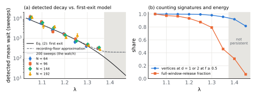
What the detector times. The decay detector first rests, taking the spread of S/N over a run’s first 200 sweeps as that run’s noise, and only then checks every five sweeps whether S/N has fallen more than three times that spread below its curled value (Table I; the “watch” of PL, Ch. 8). Its mean wait W and the first-exit prediction, compared over two decades in Fig. 3(a), are therefore distinct observables, for two reasons. First, nothing is recorded before sweep 205. For the idealized floor W = max(T,a) with exponential T of mean τ, E[W] = a + τe^−a/τ, which at a = 205 gives 462 and 265 sweeps at λ = 1.30 and 1.35, against 403–505 and 280–350 measured (the dashed curve: this floor alone, not a calibrated detector prediction). Second, the threshold is the run’s own: a torus that begins to change inside the window widens its threshold and is caught late or never, which changes both the threshold and the sample selection (Methods).

The second effect is how we read the two exceptional T24 waits at N = 64: 20,270 sweeps (λ = 1.25) and 32,155 (1.30), or 23.98 and 76.74 times the predicted first-exit means. They are not waits of a resting torus. The rows saved for those two runs record f₂₀₀ = 0.75 and 0.875 and place the 25, 50 and 75% snapshots at sweep 205, the first check after the resting window: both tori had converted three quarters or more inside the window from which the detector estimates \(\sigma_{\rm rest}\). The threshold was correspondingly low, and W records when S/N at last fell below it, from endpoints that retained energy (window releases 0.744 of 1.000 and 0.563 of 1.200 per vertex).

Dedicated tail test (T38). A prespecified tail count asked whether long waits form a second population. With w′ = W − 200 and \(\widehat\tau=\operatorname{median}(w')/\ln2\), it counts the waits k₁₀ above \(10\widehat\tau\): TAIL for k₁₀ ≥ 3, NO TAIL for k₁₀ ≤ 1, otherwise UNCLEAR. At λ = 1.25 the result is UNCLEAR at N = 64 (k₁₀ = 2; 3942 of 4000 runs recorded) and NO TAIL at N = 192 (k₁₀ = 1; 1000 of 1000); at 1.30 it is TAIL at both sizes (k₁₀ = 14, 3868 of 4000; and k₁₀ = 5, 1000 of 1000). Two TAIL cells give the registered classification TWO POPULATIONS, which stands as scored; it does not establish two physical basins. A retrospective, exploratory reading of the saved rows, made after the data were seen (no new run; Methods and Supplemental Material), uses two recorded quantities that do not depend on the detector’s threshold, f₂₀₀ and the sweep of the first sampled f ≥ 0.25, and accounts for most of it by the resting window. (i) All 190 runs without a detector crossing have f₂₀₀ ≥ 0.75 and reach f ≥ 0.25 at sweep 205: they converted inside the window and are the fastest runs, not long survivors. The tail statistic excludes them. (ii) The fastest detected waits are exits inside the window: of the runs detected within 20 sweeps of its end, 80–84% have f₂₀₀ > 0, and the fraction of all runs with f₂₀₀ > 0 is 0.144 and 0.146 at λ = 1.25 (N = 64 and 192) and 0.274 and 0.314 at 1.30, against 1 − e^−200/τ_AB = 0.211 and 0.380 for a first exit before sweep 200. (iii) The scale \(\widehat\tau\) is taken over all detected waits, those fast ones included: it is 750, 671, 267 and 238 sweeps in the four cells, against means of 917, 858, 443 and 446 for runs with f₂₀₀ = 0. The cutoff \(10\widehat\tau\) is therefore only 5.7–8.9 τ_AB, and the reference expectation ne⁻¹⁰ does not apply to it. Measured against their own mean, the f₂₀₀ = 0 runs have 0, 0, 3 and 0 waits beyond ten means, where 0.16, 0.04, 0.13 and 0.03 are expected.

That leaves three waits at λ = 1.30, N = 64 (W = 4705, 5000 and 5080). A registered replay of that cell from its seeds (T58) returns all 4,000 saved rows unchanged. For the three runs it records every five-sweep block: before detection the square count never exceeds the torus’s, no vertex reads d = 0, and the graph stays connected. One wait is the window again: an excursion inside it lowered the threshold, and three later exits that fell back went undetected. The other two read as the perfect torus at every block, for 5,000 and 4,670 sweeps. Neither registered prediction for the three held (a hidden doubly curled state; a lowered threshold in all three). Those for the cell did. Timed with no detector, the first exits of the 4,000 runs have mean 1.071±0.017 τ_AB (four standard errors above the count; Methods), one lies beyond 10τ_AB (0.18 expected), and no run ever exceeds the torus’s square count. An exploratory replay of these runs, read after every sweep, finds no sweep with more squares than the torus and separates the two: the W = 5000 run is the perfect torus through sweep 4,998 (11.9 τ_AB), while the W = 4705 run left it for three sweeps between two block readings, 7.1 τ_AB after the window. One long wait remains, which chance allows about one time in six.

A second registered run (T59) settles two points this leaves. Counted by the move in 4,000 fresh runs at the same setting, the first exit has mean 1.005±0.016 τ_AB. Read every five sweeps, the same runs give a mean later by 0.096±0.007 τ_AB, and 94% of that comes from first exits that return before the reading. The 7% belongs to the reading interval, not to the count. At λ = 1.05, where three waits near 9.5 τ_AB had appeared among 200 (Methods), 3,000 fresh move-counted first exits have means 0.992±0.023 (N = 64) and 0.946±0.031 τ_AB (N = 96), with one beyond 8τ_AB where 1.0 is expected.

Fourth map and held-out size (T60). A fourth pre-registered map uses move-level first exits and 120 replicas per cell. All 24 window cells, λ = 1.05,1.10,…,1.30 and N = 64,96,144,192, pass its stated gates and waiting-CV, local-signature and largest-component criteria. Frozen predictions for all six window settings pass at N = 288, where the conversion criteria also pass. At λ = 1.35 the largest-component criterion fails at N = 192 and 288. These are classifications by the stated criteria, not evidence sufficient to classify an equilibrium transition.

At N = 288,λ = 1.30, the mean largest-component fraction at half conversion is 0.751181, above the 0.7 threshold, but only 65 of 120 individual replicas exceed 0.7. A CV acceptance band tests one summary statistic, not the full exponential distribution. Moreover, a retrospective application of T24’s residual-wait CV criterion to the T60 rows passes all 24 smaller-size window cells too. Thus the fourth map’s success cannot be uniquely attributed to the repaired first-exit clock: the sample and diagnostic changed. The three earlier verdicts remain inconclusive.

VIII. Discussion

Side by side: in the plain-language edition this is Chapter 9, The edges and Chapter 10, What we have learned, and what comes next »

The burp belongs to the λ > 1 family. At λ = 1, which is CQG, the flat, curled and 4-cube tori are degenerate and the available decrease ε = 4(λ − 1) vanishes: the change has zero ideal-state energy difference.

The strongest quantitative kinetic result is that counting moves predicts the mean first exit with nothing fitted, consistently with directly counted exits and with the stated correction for the dearer exits left out. The energetic lower bound for sealed escape, 12 units at λ = 1.25, is certified over the tested sizes, while the available release grows with the system. Conversion snapshots support dominance by a connected flat-like region, but do not establish a unique seed or one moving boundary. Endpoint geometry is certified for the stated T8 and reached zero-energy T60 sets; the reconstructed tori remain narrow, and retained heat did not widen them in a registered test (T61). Finite-bath equilibration and geometric opening in other regimes remain open. The detected-decay tails are largely accounted for, retrospectively, by conversion inside the detector’s resting window. A replay of one cell (Sec. VII) finds one more such case and one wait of a length chance allows. Counted by the move in 7,000 fresh runs, first exits are on the count at λ = 1.05 and 1.30 with no detected excess of long waits; five-sweep readings lengthen the mean by 8–10% because some first exits return unseen. The inconclusive maps and the T38 classification are part of the result.

Relatives in condensed-matter kinetics (context, not validation). Energy-conserving conversion that ends with residual defects has relatives outside this model. In an isolated electron-lattice chain, order forms after a sudden change by nucleation and growth and can end arrested, with immobile defects, when the energy available falls below a local barrier [9]. The defects there are kinks between two symmetry-related orders, removed in pairs, and the dynamics is a physical equation of motion; neither is established here. The barrier to completing the change, which this paper does not compute, is in that literature a minimax barrier, obtained by exact enumeration on small systems and displayed as a disconnectivity graph [10].

Not claimed: that this chain is the physical time evolution of anything; a first-order transition in the thermodynamic sense; a latent heat; isotropic decompactification; a unique moving front; a general large-size law beyond the enumerated and measured sizes; an explanation for the cold-box defect count; or any rate for interchangeable (unlabelled) vertices, which would change the rates here but not the energies.

Outlook (motivation, not a result). This work is motivated by the hypothesis that space emerged from a specific ordered arrangement through a sharp change of this kind, a lattice cousin of false-vacuum decay [8], releasing a definite energy and leaving relics behind. Nothing here tests that hypothesis beyond showing classical activated escape and energy-releasing conversion in a specified graph model. No tunneling or Lorentzian spacetime dynamics has been computed. Measuring growth of both geometric periods, interfaces, and histories recorded attempt by attempt up to completion would make the next tests more discriminating.

Methods and data

Side by side: in the plain-language edition this is Chapter 9, The edges »

Sampler and validation. Simple bipartite switches preserve degree and the hard-core rule; invalid proposals are rejected. All clocks use sweeps of 2N attempts. The stationary measure follows from symmetric proposals and Metropolis detailed balance. Exhaustive small-graph checks and canonical averages validate the sampler at N = 16,18; ergodicity and equilibration at the sizes run are not proved. The square-density comparison at N = 160 agrees with Ref. [2], Fig. 8a, to rms 0.005 but differs from Ref. [3], Fig. 3, by up to 0.41 between g = 2 and 6.3. Given the differing stated protocols discussed in the Introduction, this remains an unresolved reproduction issue, not a validation of the entire uncapped equilibrium curve.

Conversion protocol. The runner advances in five-sweep blocks, recording square counts and the threshold crossings in Table I. The main conversion stage stops at f ≥ 0.98 or the configured cap; the settling stage follows even if that crossing was not reached. In T7b and T8, settling uses 600-sweep windows. The current stopping rule requires two consecutive window releases to agree within 0.005ε and the last to lie within 0.01ε of full release. Otherwise it runs to the configured settle cap. Defected endpoints can therefore exhaust the cap even when long-lived. T7 uses a fixed 300-sweep settling stretch. T7b’s nominal main and settle caps are 30,000 sweeps each; T8 uses 100,000 for each. Recorded replay configurations extend selected T7 settling caps. The frozen configuration, not the nominal duration, identifies each replay. Saved final graphs are post-settling states, whereas the 25/50/75% histograms are taken during conversion.

Analysis design. Waiting and morphology criteria for the conversion maps, and the dedicated tail-count test, were fixed before their respective runs, as were the gate, labels and cell predictions of the T58 replay (one of its three target rows already implied a lowered threshold) and of T59 (one of its seven replay targets had been replayed before registration). Endpoint-energy criteria were partly chosen after inspecting data, so the energy classification is exploratory. The Arrhenius and seed scans, the sweep-by-sweep replay, pooled distribution checks, topology certificates and interval estimates are also exploratory analyses, not independent confirmatory experiments. Identifiers such as T8 and T38 point to the configurations and analyses in the Supplemental Material. Our computational derivations remain unverified by an independent physicist.

Uncertainty and selection. Replicas, not vertices, are the independent units within a setting. We report 95% exact binomial intervals for success fractions, percentile bootstrap intervals for replica means (10,000 resamples, seed 20261009), and exponential-model intervals \([2\sum T/\chi^2_{2m,0.975},2\sum T/\chi^2_{2m,0.025}]\) for complete first-exit samples. The last are conditional on the continuous exponential approximation, not distribution-free bounds. For the T7b largest-component means, the intervals at N = 64,96,144,192 are respectively [0.983,1], [0.928,0.986], [0.906,0.995], [0.864,0.971]. The median is one in each cell, but 0, 1, 3 and 5 of the thirty individual runs have a fraction below 0.7 (0, 2, 4 and 9 in the first set). Thus a passing mean does not describe every replica. Map waiting summaries are restricted to runs reaching f ≥ 0.75; this selection can favor successful conversions. Counts of observed events, omissions and snapshot availability are given in the Supplemental Material.

Exploratory distribution checks. We divide each wait by its cell mean and compare the pooled sample with the unit exponential using the Kolmogorov–Smirnov distance D. A parametric bootstrap refits cell means in each of 10,000 simulated datasets. It reproduces the sampling grid and residual-time convention, not the threshold set by each run’s first 200 sweeps. For the 432 first exits, two of eighteen individual cells have p < 0.05, both at λ = 1.05. The 240 attempt-counted T22 exits, normalized by Eq. (2) without fitted means, give D = 0.039, p = 0.85. The Arrhenius scan reuses a seed across couplings at each size and replica. The pooled bootstrap simulates cells independently, so its 432-wait p-value does not model this dependence and is nominal. T22 includes λ in its seed derivation. For detected waits, the unfiltered T7/T8 residual sample (865 waits with W > 205) gives p = 0.03; T7 alone gives p < 10⁻³. Selecting T8 cells passing persistence, f₂₀₀ = 0 and W > 205 gives 589 waits with D = 0.030, p = 0.55. Having f₂₀₀ = 0 does not rule out an earlier exit and return. Pooling and fitting means can mask cell heterogeneity, and KS is not a decisive far-tail test. Three of 200 mixed first-exit and detected waits at λ = 1.05 exceed 75,000 sweeps (9.4–9.7 τ_AB). A registered audit (T59) replayed them from their seeds. The detected one read as the torus at every block. The two move-counted ones were offered exits A and B at 2.94–3.03 and 1.94–2.04 per sweep in every 5,000-sweep stretch, against the counted 3 and 2. With the fresh sample of Sec. VII we read the three as chance; two such first exits among 80 have probability about 10⁻⁵, computed after seeing them.

Retrospective reading of the decay rows. The reading in Sec. VII uses only columns saved by the registered runs, f_200 and the snapshot sweeps, through scripts/read_wait_detector.py. It was made after the T24 and T38 results were known, is exploratory, and changes no registered classification. A run is called perfect at sweep 200 when f₂₀₀ = 0; this does not exclude an excursion that returned inside the window. The replay (T58) reruns registered configurations from their seeds with a read-only recorder; its gate requires every saved column to return unchanged. Its detector-free first exit is the first five-sweep block at which a run no longer has S = 5N/4, X = N and every vertex at d = 1 (the basin of Table I, neutral classes included). An exit that returns within a block is not seen (the exploratory sweep-by-sweep replay of nine runs shows two), which lengthens the measured mean wait. T59 measures the lengthening for this cell, 0.096±0.007 τ_AB, by timing fresh runs by the move and by five-sweep readings together; its readers make the T22 chain’s draws in the same order and return T22’s saved first exits to the attempt. No T38 waiting-graph files are in the frozen results/ inventory, so in the three cells not replayed endpoints cannot reconstruct histories.

Companion documents. A plain-language edition (paper_plain_language.pdf, same repository) develops each concept with diagrams in the order of Secs. II–VII and links an interactive page evaluating Eqs. (1) and (2). Neither adds a result about this study.

Data and code. The source-data snapshot used for the 11 October audit is available at RecreationalPhysics, commit 5382053a. The Supplemental Material provides a claim-to-script/configuration/data map, complete check outputs and content hashes in release_manifest.json, with the analysis and figure scripts. Configurations specify seeds and durations; associated metadata record software versions but do not consistently identify the original execution commit. The endpoint certificates postdate that snapshot and are identified by the accompanying release manifest. The retrospective selection and algorithms are documented in the supplement.

Acknowledgments

The author used Claude (Anthropic) and ChatGPT/Codex (OpenAI) to assist with code, analysis and writing, and is responsible for the manuscript. We thank C. A. Trugenberger for correspondence.

References

1. C. A. Trugenberger, J. High Energy Phys. 09 (2017) 045, arXiv:1610.05934.
2. C. Kelly, C. A. Trugenberger, and F. Biancalana, Class. Quantum Grav. 36, 125012 (2019), arXiv:1901.09870.
3. C. A. Trugenberger, Networks as the fundamental constituents of the universe, J. Phys. Complex. 6, 042001 (2025), arXiv:2512.17676.
4. A. Gorsky and O. Valba, Phys. Rev. D 103, 106013 (2021), arXiv:2101.04072.
5. C. Kelly, Emergent geometry and discrete curvature in random graphs, Ph.D. thesis, Heriot-Watt University (2022), https://www.ros.hw.ac.uk/handle/10399/4591.
6. C. A. Trugenberger, Dark matter and dark energy in combinatorial quantum gravity, arXiv:2409.09385.
7. M. Creutz, Phys. Rev. Lett. 50, 1411 (1983).
8. S. Coleman, Phys. Rev. D 15, 2929 (1977).
9. H. Jang and G.-W. Chern, Suppressed coarsening after an interaction quench in the Holstein chain, arXiv:2602.05815.
10. B. B. Le, S.-H. Lee, and G.-W. Chern, Energy landscape of the kagome antiferromagnet: Characterization of multiple energy scales, arXiv:2604.18902.